Measurement issues with calculating the government budget deficit

Official measures of the government budget deficit are constructed as follows: Capture1

Where:

i =  nominal interest rate,

B = outstanding government debt,

G =  government expenditure

T = tax revenue (net of transfer payments)

Problems

1) Correction for inflation

This measure does not account for the effect of inflation – a positive rate of inflation decreases the real value of government debt even if the nominal deficit is zero.

If  Capture2 the nominal deficit will increase by  Capture3 each year, as will the nominal debt, even if the budget is balanced, but the real level of debt is unchanged

The inflation-adjusted (or real) budget deficit is the official (or nominal) measure minus the effect of inflation on existing debt:

Capture4

where r = the real interest rate.

2) Accounting for government assets

Most measures of budget deficits only account for changes in government liabilities, not changes in its assets

Some economists argue that the budget deficit should be defined as the change in government debt minus the change in government assets e.g. if a government sold one of its assets the revenue raised would then not reduce the budget deficit since the value of its assets would have fallen equivalently

However, capital budgeting it is difficult to implement since it involves deciding what government spending constitutes expenditure on capital and what does not (e.g. value of a motorway)

3) Missing government liabilities

The standard measures of budget deficits and government debt ignore many liabilities of the government

A)     future pension benefits for government workers (equal to about 50% of US debt)

B)      future social security payments (estimated to be 300% of existing US debt)

C)      contingent liabilities – when the government acts as an implicit or explicit guarantor

4) Adjustments for cyclical economic activity

The magnitude of actual government budget deficits is to a large extent dependent on the state of the economy.

During recessions incomes decline and tax revenues fall whilst unemployment increases and transfer payments rise –  leading to a worsening of public sector finances.

During booms the opposite applies and it is easier for the government budget to reach a surplus.

In order to clarify whether a change in the actual budget deficit is due to movements in fiscal policy or economic activity, the business cycle effect is netted out.

A cyclically-adjusted (or structural or full-employment) budget deficit can be calculated by estimating what the government would be spending if the economy was at its natural rate of output

Comparisons of this measure over time reflect changes in the fiscal stance of the government.

The difference between the actual deficit and the cyclically-adjusted deficit is known as the cyclical deficit. For the UK the cyclically-adjusted budget surplus in 1999-2000 was very close to the official measure (1.8%)

Types of government intervention

Type of intervention Description Example Advantage Disadvantage
Direct Provision Governments can supply public and merit goods directly to consumers free of charge. In the UK, primary school education, visits to the doctor and roads are provided free of charge. The government directly controls the supply of goods and services. E.g. It decides how many soldiers there are as it pays them directly. May potentially be inefficient  if the government produces the good itself.
Subsidised Provision The Government can pay for part of the good or service (a subsidy) but expect consumers to pay the rest. Prescriptions or dental care are subsidised in this way in the UK. Would increase the amount of the good or service, potentially to a level of which that maximises economic welfare. The decision about the level of subsidy can be ‘captured’ by producers, and so become too large to maximise economic welfare.
Regulation The Government may leave provision to the private sector but force consumers to provide a merit good. Motorists are forced to buy car insurance by law. Requires little or no taxpayers’ money to provide the good. Consumers are likely to be able to shop around in the free market for a product which gives them good value, ensuring productive and allocative efficiency. Can impose heavy costs on a poor society. Regulations can also be ignored.

If some parents had a legal obligation to pay for their children to go to school, some parents would defy the law and not give their children an education.

Are we headed for another housing bubble disaster?

Figures today show UK average house prices  have risen past the £170,000 mark for the first time since 2008. This is still nowhere near to the peak in 2007 of over £200,000 (Inflation adjusted), but the Bank of England’s commitment to low interest rates (until unemployment is below 7%), coupled with the governments help to buy scheme has led to fears of another surge in house pricing.

We now live in a culture whereby people buy houses as an investment, the value of which they expect to increase at unsustainable rates. Expectations clearly need to be adjusted.

On the banking side, more regulation needs to be enforced. The culture of reckless lending may have been simmering in the background for the last couple of years with tighter capital controls, but is by no means out of the picture. There still exists the huge moral hazard issues of the lender of last resort function, giving large banks the wrong incentives.

If anything, history tells us that we will make the same economic mistakes. Let’s hope Marc Carney has got something up his sleeve in this ‘toolkit’ of his.

Does raising tax rates necessarily raise tax revenue

When there is an income tax, the just man will pay more and the unjust less on the same amount of income.” A quote by Plato, (428BC-348BC) the famous ancient Greek philosopher. This is an early recording of behavioural psychologies towards taxation which is something I will discuss in this essay. Throughout this paper I aim firstly to see whether raising tax rates necessarily raise revenue. To do this I will look in depth at the Laffer curve and use it for my evaluation. I will also look at what factors affect how tax revenue changes when tax rates change.

To see how raising tax rates may or may not increase tax revenue, we can look at the theory of the laffer-curve.

Figure 1: laffer curve, wikipedia

Figure 1: laffer curve, wikipedia

The laffer curve shows the relationship between tax rates and tax revenue. The optimizing revenue collection tax rate (not to be confused with the optimal tax rate) is at t*, where the maximum tax revenue would be generated. The diagram theorizes that if you raise taxes above t*, then tax revenue may actually fall. This could be for a number of reasons, such as the people leaving the country or investing in tax avoidance, which I will go into greater detail on later in this essay.

Evidence of the laffer curve in practise exists from past data. Perloff gives an example by drawing on work from Fullerton (1982) and Stuart (1984). Fullerton concluded that the t* rate in America was 79% and Stuart calculated this figure at 85%. Using these figures, Perloff (2001: p.140) noted that, “Given the American t* is between 79% and 85%, the Kennedy era tax cut (from 91% to 70%) raised tax revenue and increased the work effort of top-income-bracket workers, but a Reagan era tax cut (in which the actual rate was about half as a big as t*) had the opposite effects.” The former showing the right hand side of the Laffer curve whilst the latter showing the left.

Knowing where the t* rate resides is a matter of heated debate in many countries. For example, there was a lot of controversy over the 50p tax rate in Britain, enforced in April 2010. People were worried that if the tax was enforced, it would be destructive to the economy. It was argued by the Institute of directors,  “that the new rate would damage business confidence, foreign investment and entrepreneurial aspiration.“ (BBC news, 6 April 2010) They felt that the tax would reduce long-term tax revenue and we’re not alone with this view. Looking at the diagram they were essentially saying the higher rate of tax in Britain was already at or above the t* tax rate. Figures of the revenue raised by the tax will not be published until after January 2012, however there have been recent calls by leading economists, urging the government to drop the tax at the “earliest opportunity”, claiming it is doing “lasting damage” to the economy. (BBC news, 7 September 2011)

The laffer curve theorizes that raising taxes may in fact reduce tax revenue. Capital gains tax in America, 1985 and 1994 (inflation adjusted) gives us another example of this. In 1985 the tax revenue was $36.4 billion and then in 1987 there was increase on capital gains tax. Revenue from this tax declined after this and in 1994 the revenue fell by .2 billion to $36.2 billion, “even though the economy was larger, the tax rate was higher, and the stock market was stronger in 1994.” (Jim Saxton, 1997)

A well known advocate of the laffer-curve,  a man called William Kurt Hauser, created a theory that is known as ‘Hauser’s Law’. This states that “federal tax revenues since World War II have always been approximately equal to 19.5% of GDP, regardless of wide fluctuations in the marginal tax rate.”(Wikipedia, 2011) Hauser’s law is important, as it gives us some empirical evidence of the principle behind the laffer-curve.

Figure 2: Hauser's law (from J.D. Tuccille, tuccille.com)

Figure 2: Hauser’s law (from J.D. Tuccille, tuccille.com)

Looking at the graph above we can see the top individual tax bracket in comparison to the revenue as  a percentage of GDP. We can clearly see that no matter what the marginal tax rate of the top income earners has been, revenue as a percentage of GDP has be steadily fluctuating around 18-20%. This shows that raising tax rates does not always raise tax revenue.

There are some criticisms of Hauser’s law as well as the laffer curve. Daniel J. Mitchell, a columnist for Forbes.com, argues that Hauser’s law is in existence in America because they have a federalist tax system unlike lots of countries in Europe who have a national sales tax (V.A.T), and also because they have a more progressive tax system. He believes the tax system in America represents a political trend and so Hauser’s law essentially does not represent true economic law. (Daniel J. Mitchell, 2010) The main criticism of the Laffer curve is to do with its shape as no-one truly knows how It looks. It is also argued that at 100% taxation, revenue will not necessarily be 0, as some people work for charities and other enjoy their jobs etc.

We can construe from these criticisms that if Hauser’s law only exists in the USA, then perhaps that is because of their tax composition and therefore, the types of taxes that a government pursues effects how much revenue is raised with a tax increase/decrease. I will discuss the shape of the laffer curve further on in the essay and will now go on to explain the factors which affect how tax revenue changes with tax rate changes.

In 2006, a report by Louis Levy-Garboua, David Masclet and Claude Montmarquette for Quebec’s Centre Interuniversitaire de Recherche en Analyse des Organisations (CIRANO) looked at behavioural factors affecting tax revenue. They came to the overall conclusion that “The Laffer curve arises both from asymmetry of equitable rewards and punishments and from the presence of a substantial share of emotional rejections of unfair taxation.” (Louis Levy-Garboua, David Masclet, Claude Montmarquette, 2006)

They say that the Laffer curve is caused by unfair rises in taxation which are considered personal and make people more likely to try to find ways to avoid paying their taxes. When taxes are perceived as exogenous and impersonal, they feel that the Laffer curve does not kick in. This suggests again that different types of taxes are more or less likely to raise revenue than others. Perhaps, for example, a ‘stealth tax’ which is used by governments to increase their revenues without raising the ire of taxpayers is a better method to raising revenue than by increasing a more direct and personal tax, such as income tax.

Kurt Brouwer also talks about how behaviour affects how tax revenue changes when tax rates change. He gives an example using capital gains tax. Capital gains tax is a “tax on the profit or gain you make when you sell or ‘dispose of’ an asset.”  For example, if you bought credit default swaps for £5000 and then sold them next year for £12000, you’ve made a gain of £7000 and this is the figure that will be taxed. (HM revenue and customs) Brouwer argues that there is a clear correlation between capital gains tax and the realization of gains. He says, “when capital gains tax rates go up, investors slow down realization of gains. So, despite a higher capital gains tax rate, the actual revenue received from capital gains taxes may not go up much.” And vice versa.  He argues that overall, an increase in tax rates may not actually increase tax revenue. (Kurt Brouwer, 2010)

David Ranson, the head of research at H.C. Wainwright & Co. Economics Inc, again, talks about behaviour towards taxation saying, “Raising taxes encourages taxpayers to shift, hide, and underreport income. . . . Higher taxes reduce the incentives to work, produce, invest and save, thereby dampening overall economic activity and job creation.” He suggests that rather than looking at taxation to increase revenue, we should look at increasing GDP. (David Ranson, 2008)

Ranson, Brouwer and the report from CIRANO all speak about behavioural psychologies towards taxation. When taxes are raised above a certain level people may be more likely to change their behaviour. If the taxes are seen as high and unjustly so, then perhaps for example, people will invest more into tax avoidance, convert more income into capital gains, have reduced incentives to work, or even leave the country. We can deduce that the populace behaviour has an impact on how tax revenue changes with a rise in taxation.

Another issue discussed briefly before in this essay which affects how tax revenue changes with tax rate changes is the composition of the Laffer curve. Although it is widely accepted that there will be no tax revenue at 0% taxation and (although disputed in some cases) at 100% taxation, it is unclear as to what the Laffer curve actually looks like, and it is more than likely that it differs from country to country because of different views and behaviours towards taxation.
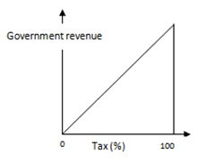
Figure 3

Figure 3

For an example, If we had a Laffer curve which looked like the one I have drawn above (Figure 3), it would be beneficial for a government to tax up to 99%, as tax revenue would keep rising up until this point. However, If we had a Laffer curve which looked more like Figure 1, then taxing above 50% would cause revenue to fall. Therefore the composition of the Laffer curve is a huge factor in how raising taxes would affect tax revenue. As I have previously stated; exactly where the t* rate lies and what the Laffer curve looks like is heavily debated. Looking at figure 2 again we can say that the t* rate in America should be the smallest value at which the revenue raised is around 18-20% of GDP. Going above this figure will not raise anymore taxes and it is possible that it will needlessly cause GDP to fall.

For another example to see what factors affect whether raising taxes increase tax revenue, we can look at the backwards bending supply of labour curve.

Figure 4: Taken From W.Morgan, M.Katz and H.Rosen, (Microeconomics, 2009)

Figure 4: W.Morgan, M.Katz and H.Rosen, (Microeconomics, 2009)

Looking at the diagram A (above), the budget lines shows us different wage rates. At the bottom wage rate (slope = -w3), according to the indifference curve, the amount of leisure and consumption that will be consumed is e3. As we move up the wage rates to we can see that the first shift causes the endowment point to change to e2, where the consumer works more than before, however as we move up to the next wage rate we can see that at e3, the consumer starts to work less.  We can explain this by talking about income and substitution effects. (W.Morgan, M.Katz and H.Rosen, 2009)

The income effect shows us the change in consumption due to a change in the consumers income and the substitution effect shows us how a change in income changes the supply of labour. Looking at figure 1, diagram A we can see that these two effects are opposite. From e1 to e2 the income effect is dominating the substitution effect. At this point people would rather increase their consumption than leisure,  as consumption rises more than hours of leisure. However, from endowment e2 to e3, people would rather have more hours of leisure than consumption. The substitution effect dominates the income effect. (W.Morgan, M.Katz and H.Rosen, 2009)

From this evaluation you can see how figure 1, diagram B is formed. As first as wages rise, people work more until the wage rate rises above a certain point and people decide to reduce hours. Thinking about taxation, people will work more if the tax rate rises when they are in the backwards bending section of their labour supply curves as real wages fall. However, as the tax rises further, workers will be in the upward sloping section, and therefore an increase in the tax will reduce the number of hours worked. The optimizing revenue  tax rate will be where the most hours are worked as this will produce the most amount of tax revenue. We can say that the size of the income and substitution affect has a impact on how much revenue will be raised with a rise in taxation.

I do not however feel that the backwards bending supply of labour curve shown necessarily shows the whole picture. For example, if you raise income tax it’s essentially a cut in real wages so (according to the diagram) you should work less if you are in the upwards-sloping section. However in reality most people have a contracted amount of hours and so whilst it may be easier to get over-time, to work less may not be an option for many people. Therefore I believe the curve should more inelastic and though the substitution and income effects will have some effect, I feel the that the effects are limited.

To conclude, raising taxes does not necessarily raise tax revenue. I have shown using theoretical analysis of the Laffer curve  that if a tax is above the optimizing revenue rate, then an increase in taxation can actually cause a reduction in tax revenue. I have also backed up this theory with empirical evidence.

The first factor I have talked about which affects how tax revenues change with tax rates is behaviour. People respond in different ways to taxation and depending on how they respond, more or less tax revenue will be seen as a result of increase or decrease in tax rates. I also believe that the type of tax can cause different reactions as the 2006 report from CIRANO pointed out as well as conclusions surrounding Hauser’s Law. I have also talked about the income and substitution effects which link in with behaviour. Depending on how large each affect is and what the wage rate currently is at, people will respond accordingly. For example, if an increase in taxation caused people to give up hours of work for leisure then tax revenue may fall and vice versa, although as I have stated, I feel these effects are limited.

I also talked about the composition of the Laffer curve.  Depending on what it looks like, and where the current taxation level resides, revenues could rise or fall with tax increases or decreases. Again, it can be said that the make-up of this curve can be related to the populace behaviour because exactly where the t* rate lies, depends on where people start reacting to tax rates. Finally, I stated the type of tax has an impact on revenue raised. However after researching I felt that there was a lack of data and that I could not confidently come to a conclusion about how revenue changes with specific taxes

Therefore, although I may have not covered all the factors affecting how tax revenues change with tax rates, I feel the main factor is populace behaviour. Populace behaviour entails how big the substitution and income effects are, the composition of the laffer and also how people react to certain types of taxation.

References

David Ranson, (2008) You Can’t Soak the Rich

BBC news. (06/04/2010) New 50% tax rate comes into force for top earners [Online] Available at: <http://news.bbc.co.uk/1/hi/uk/8604215.stm> [Accessed 22/12/2011]

BBC news. (07/09/2011) Top 50p tax rate damages UK, says economists [Online] Available at: <http://www.bbc.co.uk/news/business-14810323> [Accessed 22/12/2011]

Jim Saxton. (1997) The Economic Effects of a Capital Gains Taxation, [Online] Available at: <http://www.house.gov/jec/fiscal/tx-grwth/capgain/capgain.htm> [Accessed 22/12/2011]

Wikipedia. (last edited 2011) Hauser’s law, [Online] Available at:  <http://en.wikipedia.org/wiki/Hauser’s_law> [Accessed 22/12/2011]

Daniel J. Mitchell. (2010) Will “Hauser’s Law” Protect Us from Revenue-Hungry Politicians? [Online]Available at: <http://www.forbes.com/sites/beltway/2010/05/21/will-hausers-law-protect-us-from-revenue-hungry-politicians/> [Accessed 22/12/2011]

Louis Levy-Garboua, David Masclet, Claude Montmarquette (2006) A Micro-foundation for the Laffer Curve In a Real Effort Experiment. [Online]Available at: <http://www.cirano.qc.ca/pdf/publication/2006s-03.pdf>  [Accessed 22/12/2011]

HM revenue and customs, [Online] Available at: <http://www.hmrc.gov.uk/cgt/intro/basics.htm#1> [Accessed 22/12/2011]

Kurt Brouwer, (2010) Does hiking tax rates raise more revenue? [Online]Available at: <http://blogs.marketwatch.com/fundmastery/2010/07/02/does-hiking-tax-rates-raise-more-revenue/>  [Accessed 22/12/2011]

Jeffery M. Perloff, 2001: Microeconomics. USA: Addison Wesley Longman, Inc. P.40.

Wyn Morgan, Michael Katz and Harvey Rosen, (2009) Microeconomics – 2nd European Edition. New York, McGraw-Hill Education (UK) limited.

Figure 1: http://en.wikipedia.org/wiki/File:Laffer-Curve.svg

Figure 2: J.D. Tuccille, Hauser’s Law, the Laffer curve and pissed-off taxpayers [Online] Available at: <http://www.tuccille.com/blog/2008/05/hausers-law-laffer-curve-and-pissed-off.html> [Accessed 22/12/2011]

Figure 4: Wyn Morgan, Michael Katz and Harvey Rosen, 2009: Microeconomics – 2nd European Edition. New York, McGraw-Hill Education (UK) limited. P. 146.

Should the United Kingdom remain in the EU (brief)

Pros Cons
Free markets – especially good for the service industry who find it easier to access more customers. To an extent, the EU is undemocratic and unaccountable – the closest a regular citizen can come to affecting policy is by voting for their MEP.
EU is a form of wealth distribution – Britain is the third biggest contributor to the EU (2011), it pays more than other countries because it is richer. Free trade could still be possible without being a member of the EU. The EFTA, EEC or individual treaties could be passed to keep free trade with Europe if countries comply.
Britain joined the economic community of the EU in 1973 after learning that trade with the commonwealth was not as lucrative as originally thought Costs the UK taxpayers a lot of money – “When you take into account additional revenues raised from customs duties, agricultural levies, VAT and even sugar contributions, Britain handed over a total of €13.825bn to Brussels last year.” We do of course receive money back but this is still a vast sum of money which could arguably be put to better use in the UK’s wavering economy.
If we leave, the Trans-national (TNCs) may leave also – its estimated around 3 million jobs would be lost from companies such as Nissan who make good use of the cheap exports to other EU countries. In ‘06’ 45% of the EU spending was on CAP which employs just 5% of EU citizens and generates only 1.6% of the GDP. In 2012 spending on CAP is still huge at around 33%
Trade – around 52% of total traded goods from the UK is with the EU. Immigration – 27% of total net migration in 2010 was from EU which Britain could control if out of the EU. Free NHS to EU members costs the UK lots of money from people who have never or barely paid into the system – this not only causes increased costs but also increases waiting time.
Influence in Brussels which may not be seen if we leave the EU. EU regulation restricts small and medium sized firms which may boom without these restrictions.
Tuition fees for British citizens in other EU countries are cheaper as a result of being in the European Union.


The legalities of joining the EU can be argued. Gordon Brown voted for the Lisbon treaty after citizens were not given the promised referendum from the labour party.


Sources

http://www.telegraph.co.uk/finance/financialcrisis/9643193/EU-budget-who-pays-what-and-how-it-is-spent.html

http://www.bbc.co.uk/news/uk-politics-20448450

http://www.bbc.co.uk/news/uk-politics-11645975

The East Asian Financial Crisis of 1997 (A brief overview)

en.wikipedia.org

en.wikipedia.org


From the 1960s to 1990s the performance of the East Asian economies was somewhat spectacular. Their global share of GDP was consistently increasing against the rest of the world, almost doubling in the space of 30 years to around 22.5% in 1990. However, there were apparent weaknesses in their financial structure which can partly explain the cause of 1997 East Asian Financial crisis.

Success story

Until 1997 the countries of east Asia had very high growth rates

The ingredients for their success included but were not limited to: High saving and investment rates, a strong emphasis on education, a stable macroeconomic environment, freedom from high inflation or economic slumps and a highs share of trade in GDP.

Weaknesses

The main weaknesses that became apparent were:

Productivity – Rapid growth of inputs yet little increase in the productivity rate (little increase in output per unit of input)

Banking regulation – poor state of the banking regulation

Legal framework – lack of a good legal framework for dealing with companies in trouble

The Crisis

During the 1990’s there was lots of speculation on the Thai baht as property markets were heating up. After running out of foreign reserves Thailand had to float their currency, cutting its peg to the US $. The crisis started on July 2, 1997 with the collapse of the Thai baht. The sharp drop in currency was followed by speculation against the currencies of Malaysia, Indonesia, Philippines and South Korea. All of the afflicted countries sought out the IMF for assistance apart from Malaysia.

Debt-to-GDP ratios rose drastically as exchange rates fell. Interest rates of 32% in the Philippines and 65% in Indonesia over the crisis did nothing to calm investors and both countries saw a greater percentage decrease in GNP and exchange rate (against the US $) than  South Korea.

It was not exactly clear what sparked the ignition of the crisis. The first major corporate failure was in Korea when Hanbo steel collapsed under huge debts. This was soon followed by Steel motors and Kia motors which meant problems for local merchant banks who had borrowed from foreign banks.

Local banks were hit with: withdrawal of foreign funds, substantial foreign exchange losses, sharp increase in NPL’s (non performing loans) and losses on equity holdings.

Pilbeam argued the crisis was due to the banking system and its relationship with the government and corporate structure rather than macroeconomic fundamentals.

The countries wanted high economic growth and so applied pressure on firms to make large investments and on domestic banks to lend to firms. These domestic banks failed to assess the risks properly and financed the loans from residents, foreign banks and investors. These loans were also guaranteed by the government. Overall the banking system was weak, with poor regulation, low capital ratios, poor selection schemes and corruption. Thus the banks lent to firms without a regard for profitability, explaining the large number of non performing loans.

The downturn of the crisis was ‘V-shaped’ – after the sharp output contraction in 1998, growth returned in 1999 as depreciated currencies spurred higher exports.

External Factors

Japans recession through 1990’s – kept interest rates low which allowed for East Asian economies to easily finance excessive investment projects.

50% devaluation of the Chinese currency in 1994 – can partly explain the loss of cost competitiveness from the East Asian economies

Financial deregulation and Moral hazard – attracted foreign banks to invest, more so because of the government guarantee which allowed for the banks’ reckless loan making.

Sharp appreciation of the dollar from mid 1995 – led to deterioration of economies who had pegged their currencies to the dollar. Given time lags between exchange rate effects and trade, this began to affect their export performance in 1996/97.

The IMF

Objectives: prevention of default, prevention of free fall exchange rate, prevention of inflation, maintenance of fiscal discipline, restoration of investor confidence, structural reform of financial sector and banking system, structural reform of corporate sector, rebuilding of foreign reserves, limiting the decline of output.

At their disposal they had the following tools: bank closures, fiscal/monetary discipline and structural reform of the banking and corporate sector.

Did the policies work?

Policies were harsh and depend crisis

Closure of banks reduced credit and created panic for international investors which led to bank runs

Higher interest rates and tighter fiscal policy reduced output. The tight fiscal policy was viewed as harsh considering most countries were already running a fiscal surplus.

There is an argument that knowing the IMF was there to help could have worsened the problem of moral hazard.

Post crisis?

Output fell and there was a fiscal deficit. The current account improved, due to fall in imports and rise in exports after devaluation. Savings increased and investment fell. Overall the recession was short and the economies recovered quickly. This was largely to do with the boost in exports caused by the devaluation.

Insurance companies and risk neutrality

The requirements for the insurance market to be efficient are that the least risk adverse agent bears all the risk. This means that the agents will be bearing all the risk giving the insurance company a more certain outcome.

The market will also have to be in equilibrium, which means that two conditions will be have to be met. The first is the break even condition; this means that no contract makes negative profits. If the insurance company is not making profit off of a contract then this is inefficient and may mean the company would have to shut down depending on the profit made from other contracts. The market will also have an absence of unexploited opportunities for profit. If this is not that case then rival companies can exploit this opportunity and offer a better contract.

To be efficient the insurance market a firm will also have to be in perfect competition so they can offer a fair insurance (Risk premium = PR of loss x loss). If they do not offer fair insurance, another company can under-cut them and steal all their customers.

Finally, the market will need to have perfect information so they can offer the correct premium to everyone. Otherwise they will have to pool equilibrium as they will not know individual risk types. This would mean low risk people will be essentially paying for part of the high risk candidates insurance as well as their own which is not Pareto efficient. Pareto efficiency is when principal cannot be made better off without making the agent worse off. This condition must be met for the market to be efficient. If it is not met then they will be at a point where both parties can be made better off.

The insurance markets pretty much meet all the requirements above and so to an extent are efficient. Although of course perfect information is not quite possible.  Insurance companies reduce the amount moral hazard and adverse selection in the market by for example, making candidates fill out forms which void contracts if  information proves to be false and offer no claims bonuses.

To discuss whether risk neutrality is a necessary and sufficient condition for insurance to take place, we need to look at what would happen in the three possible scenarios: risk neutral, risk adverse and risk loving.

We can start by looking at a risk-neutral insurance company. In reality, large organisations such as insurance companies tend to be risk neutral for mainly two reasons: the risks are small relative to the organisations size and as they offer so many risk contracts, on average they all tend to cancel each other out. A risk neutral insurance company earn their profit from the fact that the value of premiums they receive is either greater than or equal to the expected value of the loss.

Even insurance companies that take on purely risky customers will still be risk neutral as they will raise the premiums to offset the extra risk. For example, some specialist  holiday insurance companies may only take on candidates who already have pre-existing medical conditions and find it difficult to get insured elsewhere. The companies will offset the extra risk however by charging much higher premiums. Again the value of premiums they receive will be either greater than or equal to the expected value of the loss.

An insurance company cannot be risk averse because of the nature of the insurance market. If the company is risk averse, then it will charge premiums much higher than the expected value of the loss. In the presence of perfect information and perfect competition, customers will not choose to insure with this company as there will be better alternatives elsewhere. Therefore the if the insurance company was risk averse it would get no customers and soon fail.

Finally, an insurance company will not work in the long run if it is risk loving. A risk loving firm would accept lower premiums from customers than a risk neutral firm would and hope that the gamble pays off. This would mean that they would be expected to make a loss overall as their premiums would be less than their expected loss. Therefore eventually they would be making a negative profit and would have to shut down. (Unless they are very, very lucky!)

So for all of these reasons, it’s necessary for an insurance company to be risk neutral for insurance to take place. It is also a sufficient condition for insurance to take place as they will be at a minimum, breaking even and so can continue to exist in a perfectly competitive market, and they can offer a competitive premium to survive in a market with perfect information. Being risk neutral will also allow the insurance company to be efficient, as they will be making the break even condition.

Project crashing – a few considerations

Firstly, what exactly is “crashing” an activity? Put simply, crashing an activity is the act of shortening the  overall project duration by reducing the time of a critical activity. A critical activity is an activity which must start and finish on time for the overall project to be completed on time.

There are many practical factors which a company should take into account before deciding to crash an activity. Also, depending on the type of company and project, these factors may vary.

The first consideration should be if crashing an activity will make you any money. Even if the money saved does not outweigh the cost of finishing early, crashing may still make you money by freeing up yours and your teams time to focus on other projects.

We also need to know if workers are available to do the overtime. If so, are these workers happy to do the overtime and will working this overtime makes them less productive in the following days of the project? If the project involved heavy manual labour for example, then working extra days may tire the workers out and make them less productive. Pushing the workers to do more may also increase the risk of injuries that could cause further delays. If you need to bring in extra resources to crash the project then they may not be familiar with the task at hand. Therefore you may need to train them and they may be less efficient than the current resources.

If an activity is crashed then there may be an increased risk of missing a deadline because of reduced slack. Missing deadlines may hamper client relations and so be detrimental to the business. Finishing a project on time may also be detrimental. For instance, if a company was running a stock audit for a retailer, then finishing early may make it appear as if they have cut corners in counting.

Another practical factor you would need to look at is if there are the materials available to crash an activity. If the materials will only be delivered at a certain time then crashing may not be an option.

If the company is working on multiple projects then will crashing one activity mean other projects are delayed. There may also be legal considerations to take into account, i.e. the maximum hours of the working week for staff.

Finally, before crashing an activity, a company should look at whether there are there other options to crashing which is more cost or time effective. Fast tracking is another viable option where you overlap tasks which were initially scheduled sequentially. You could also make other activities more efficient, by for example, splitting up a long task into smaller intervals as people may work harder in a short space of time than if they have to pace themselves to work a full day.

Are the assumptions of the Marshallian and Hicksian consumer optimisation problems plausible?

The assumptions made implicitly in the two models relate to the basic axioms of consumer theory which I have briefly described below.

Completeness – “for any pair of bundles, our consumer can say if one of the pairs is preferred to the other or is indifferent.” (M. Hoskins, pages 3)

Transitivity – “if APB and BPC then APC”. Also works with indifference – if A/B (A indifferent to B) and B/C then A/B (M. Hoskins, pages 4)

Continuity of preference – “for any bundle of goods, this requires another bundle ‘near it’ such that these two bundles and indifferent to each other.”  “This requires the divisibility of goods and allows us to define the marginal rate of substitution between x and y.” (M. Hoskins, pages 4)

Non satiation – “consumers always prefer more goods to fewer. This deduces that indifference curves slop down from left to right.” (M. Hoskins, pages 5)

Convexity of preference – “people prefer a mixture of bundles.” “This leads to the diminishing marginal rates of substitution. “(M. Hoskins, pages 7)

The assumptions are mainly the same for both the Hicksian and Marshallian consumer optimisation problems. We assume that both optimisation problems have the traits of completeness and transitivity as otherwise we would not know the consumers utility to work from. These two traits however can be seen an irrational when related to the real world. There may be situations in which decision making can be extremely difficult and so a consumer may not be able to decide if a bundle of goods are preferred to another or indifferent, rendering us unable to economically analyse the situation using this model. Also, it assumes that the customer knows their utility that they will receive from the product which is not always the case. The transitivity assumptions eliminate the possibility of intersecting indifference curves. At any one point in time, this could be true, for example, today I may prefer an apple to pear and a pear to an orange, and therefore I would prefer an apple to an orange. However, it does not take into account the time horizon. Tomorrow my preferences may change, and neither model takes that into account.

Continuity of preference is also assumed by both models and both assume that the marginal rate of substitution equals the price ratio (P1/P2). This however ignores quantity discounts; if you order in bulk then you are likely to get more for you money.

The non-satiation property also will not hold in reality. The consumer is always defined as per period and there is usually an upper limit on consumption of most goods in a specific time frame. This assumption also links in with the other assumption made in both models that that X1*>0 and X2*>0 (non-negativity). If there are two goods, for example, carrots and peas and the consumer does not like carrots, he does not prefer to have more as he does not like them. What also if one of the goods was pollution, which it would be rational to prefer none of.

The last assumption of the basic axioms I have listed is the convexity of preference which again for reasons listed before, may not hold in reality. People may prefer a mixture of bundles in some cases, but not in others. If they do prefer the mixture of goods then the diminishing marginal rates of substitution does makes sense in reality. For example, if the two goods were coke and water (and you preferred a mixture of the two) and you had loads of water and no coke, then eventually the enjoyment you would gain from an extra glass of water would fall. You would therefore be prepared to lose more water in comparison to the amount of coke you would gain.

Although the two optimisation problems share all the assumptions above, they also have individual assumptions. The Marshallian optimisation problem specifically assumes that the customer is a utility maximiser. This is in line with the rational theory of the consumer as he wants to maximise his utility according to his wealth. This is not always true of reality as it will depend on the type of consumer. Some consumers may well try to maximise their utility but this will mean exhausting income. For example, people who are hooked on drugs may spend all of the income on drugs which they believe gives them their maximum utility. Other consumers will want to save some of their income and in doing so happily forfeit the extra utility.

Finally, the Hicksian optimisation problem assumes that the consumer targets a utility and finds the most cost effective way to reach this. I think this is probably truer of reality than the Marshallian method; however again, it depends entirely on the consumer himself. Less wealthy consumers may decide they want a certain product and then search the internet and high street to find the best deal. A consumer who is a billionaire however may not have a target utility as money is not a worry. He may also not adhere to price ratios – if a good increases in price, he may buy more of that good as a symbol of status.

A comparison of the Gini and Atkinson Measures of Inequality

The Gini and Atkinson Indexes are both measures of inequality. The Gini measure however is a positive measure, whilst the Atkinson is a normative measure. A positive measure is purely statistical whereas a normative measure is “based on an explicit formulation of social welfare and the loss incurred from unequal distribution.”[1]

The Gini coefficient measures inequality using values of a frequency distribution. It is derived from the Lorenz curve framework. If the Lorenz curve is equal to zero, then it will be equal to the line of equality and everyone will have the same income. The more the curve deviates from the line of equality, the higher the inequality. Gini coefficients can be used to compare income distribution over time, making it possible to see how inequality changes over a period independent of absolute incomes.[2]

The main weakness of the index as a measure of income distribution is that it cannot differentiate between different kinds of inequalities. Theoretically, two Lorenz curves could intersect one another (showing different patterns of income inequality) but still result in a similar Gini coefficient. The Gini coefficient measures relative and not absolute wealth. Therefore, when a Gini coefficient of a developing country rises, this could be misleading. Changing income inequality by Gini coefficients may be down to things such as structural changes or immigration. A rising Gini coefficient suggests increasing inequality but it could be the case the number of people in the absolute poverty bracket actually decreases. Economies with similar incomes but different income distributions can actually have the same Gini index. For example, one economy has 50% of people with no income and the other 50% having equal income, giving a Gini index of 0.5. Another economy has 75% of the lowest income earning people with 25% of income while the other 25% of people have 75% of income which also gives a Gini index of 0.5. [3] Clearly the Gini coefficient will not always necessarily capture the whole picture about inequality within an economy.

Because of these limitations of the Gini coefficient, other methods can be used in combination or separately. For example, entropy measures such as the Atkinson index can be utilised.

The Atkinson measure allows for different parts of the income distribution to have certain levels of sensitivity to inequality. It incorporates a sensitivity parameter which allows the researcher to attach a weight to inequality at different points. Atkinson when creating the model was especially concerned with how the Gini measure could not place different weights on certain income brackets.[4]


In his paper ‘On the Measurement of Inequality’ Anthony B. Atkinson compared inequality in seven advanced and five developing countries. He compared three conventional measures (one of which was the Gini coefficient) against three differently weighted Atkinson indexes; the weight was increasing on poorer end of the scale. This data only highlighted the differences in the measures. With a weight of ε = 2 attached to the lower income scale, the Atkinson measure disagreed with the Gini coefficient in 17 cases. With ε = 1, a smaller inequality aversion, the Atkinson measure still disagreed in 5 cases. The results show that conclusions reached about income inequality is dependent on the level of inequality aversion. The reason for this is to do with the distribution of income. In developing countries, incomes are more equal at the lower end of the scale and less equal at the top than in developing countries. As we increase inequality aversion, more weight is placed upon the lower end of the scale causing distortions.[5]

The main difference between the two measures is therefore this sensitivity parameter. This parameter makes the Atkinson subjective whereas the Gini measure is objective.[6] While perhaps yielding a similar result when a low level of inequality aversion in the Atkinson measure is used, clearly by manipulating the Atkinson measure, results can differ greatly between the two. It is subjective because the user can choose what subgroups to weight more heavily than others. The Atkinson index is also subgroup consistent, this means if in a subgroup, inequality declines ceteris paribus, then overall inequality declines. It is also decomposable, which means the total inequality can be broken down to a weighted average of the inequality which exists within the subgroups. These two qualities are something which the Gini coefficient does not hold. The Gini coefficient gives an equal weight to the entire distribution but the Atkinson index gives more weight to the lower end of the distribution, this means it accounts more wholly for things such as income poverty and illiteracy.[7]